🧬 DNBelab C Series HT scRNA Analysis Pipeline

📋 Overview

This document provides a complete guide on how to use dnbc4tools for single-cell RNA sequencing data analysis.

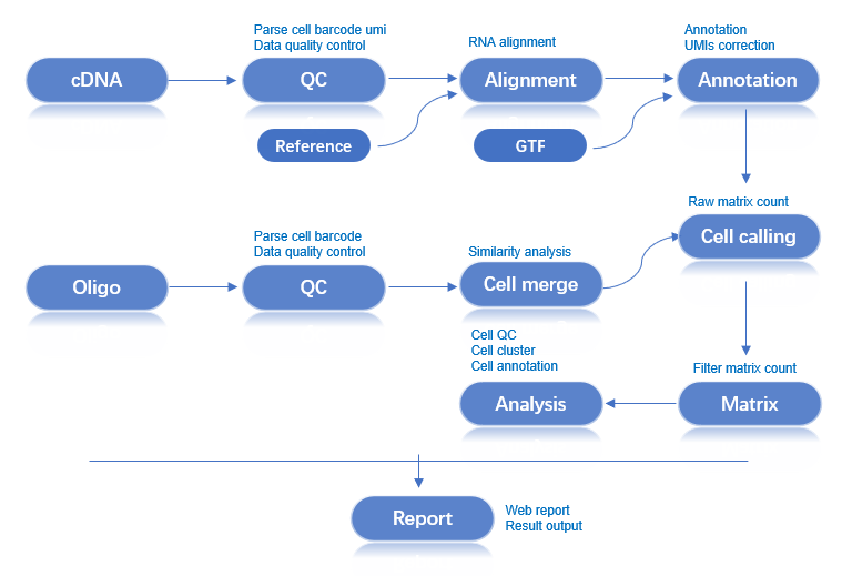
Workflow: Raw Data → Quality Control → Alignment → Cell Identification → Expression Matrix → Analysis Report

📁 File Preparation

Two types of FASTQ files are required for the analysis:

📊 Reference Data

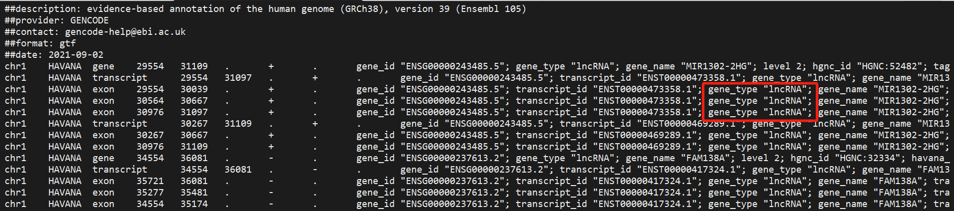
File Requirements

GTF File Requirements:

• Must contain annotations of type "gene" or "transcript" as well as "exon".
• Attributes must include "gene_id" or "gene_name" and "transcript_id" or "transcript_name".
• The GFF file format is not supported.
• The genome file and annotation file must be from corresponding versions.

GTF File Processing (Optional)

GTF files downloaded from sites like ENSEMBL and UCSC often contain many types of genes. Selecting specific gene types relevant to your research can reduce overlapping gene annotations and improve the uniqueness of alignments, as reads mapping non-uniquely to multiple genes are filtered out.

We provide three functions for GTF file processing:

Gene Type Statistics

# Count gene type quantities
$dnbc4tools tools mkgtf \
  --action stat \
  --ingtf genes.gtf \
  --output gtfstat.txt \
  --type gene_biotype

Example Output:

$cat gtf_type.txt
Type    Count
protein_coding  20006
lncRNA  17755
processed_pseudogene    10159
unprocessed_pseudogene  2605
misc_RNA        2221
snRNA   1910
miRNA   1879
TEC     1056
transcribed_unprocessed_pseudogene      950
snoRNA  943
transcribed_processed_pseudogene        503
rRNA_pseudogene 497
IG_V_pseudogene 187
transcribed_unitary_pseudogene  146
IG_V_gene       145
......

Correct GTF File

If a GTF file has incomplete content, the main analysis pipeline may fail due to incomplete annotations. This function can automatically fill in missing information in gene and transcript entries to ensure the pipeline runs smoothly.

# Correct GTF file
$dnbc4tools tools mkgtf \
  --action check \
  --ingtf genes.gtf \
  --output corrected.gtf

The software cross-references gene_id with gene_name and transcript_id with transcript_name to fill in missing details and flags locations where multiple gene information might exist.

Filter Gene Types

# Filter gene types
$dnbc4tools tools mkgtf \
  --ingtf genes.gtf \
  --output genes.filter.gtf \
  --type gene_biotype

Default included gene types:

protein_coding
lncRNA/lincRNA
antisense
IG_V_gene
IG_LV_gene
IG_D_gene
IG_J_gene
IG_C_gene
IG_V_pseudogene
IG_J_pseudogene
IG_C_pseudogene
TR_V_gene
TR_D_gene
TR_J_gene
TR_C_gene

You can also use the include parameter to customize the gene types to be retained:

# Custom gene type filtering
$dnbc4tools tools mkgtf \
  --ingtf genes.gtf \
  --output genes.filter.gtf \
  --type gene_biotype \
  --include protein_coding,lncRNA,lincRNA,\
        antisense,IG_V_gene,IG_LV_gene,IG_J_gene,\
        IG_C_gene,IG_V_pseudogene,IG_J_pseudogene,\
        IG_C_pseudogene,TR_V_gene,TR_D_gene,TR_J_gene,TR_C_gene

Build Reference Database

Before running the dnbc4tools rna run analysis, a reference database must be built. This step uses the annotation file (GTF) and reference genome (FASTA) to create an index for aligning and annotating the sequencing reads.

# Build reference database
$dnbc4tools rna mkref \
  --fasta genome.fa \
  --ingtf genes.gtf \
  --species Homo_sapiens \
  --threads 10

Output:

Upon successful execution, a reference database directory will be created at the specified location with the following structure:

/opt/database/Homo_sapiens
├── fasta
│   ├── genome.fa
│   └── genome.fa.fai
├── genes
│   └── genes.gtf
├── ref.json
└── star
    ├── chrLength.txt
    ├── chrNameLength.txt
    ├── chrName.txt
    ├── chrStart.txt
    ├── exonGeTrInfo.tab
    ├── exonInfo.tab
    ├── geneInfo.tab
    ├── Genome
    ├── genomeParameters.txt
    ├── mtgene.list
    ├── SA
    ├── SAindex
    ├── sjdbInfo.txt
    ├── sjdbList.fromGTF.out.tab
    ├── sjdbList.out.tab
    └── transcriptInfo.tab

The ref.json file records the main information of the database.

{
    "chrmt": "chrM",
    "genome": "/opt/database/Homo_sapiens/fasta/genome.fa",
    "genomeDir": "/opt/database/Homo_sapiens/star",
    "gtf": "/opt/database/Homo_sapiens/genes/genes.gtf",
    "input_fasta_files": [
        "genome.fa"
    ],
    "input_gtf_files": [
        "genes.filter.gtf"
    ],
    "mtgenes": "/opt/database/Homo_sapiens/star/mtgene.list",
    "species": "Homo_sapiens",
    "version": "dnbc4tools 3.0beta"
}

The following information will be printed during runtime:

Creating new reference folder at /opt/database/Homo_sapiens
...done

Writing genome FASTA file into reference folder...
...done

Indexing genome FASTA file...
...done

Writing genes GTF file into reference folder...
...done

Generating STAR genome index...
...done.

Writing Reference JSON file into reference folder...
...done

Analysis Complete

🚀 Main Pipeline

Multi-Sample Batch Processing (Optional)

To simplify the analysis of multiple samples, you can use a configuration file to generate a shell script for each sample.

$dnbc4tools rna multi \
  --list sample.tsv \
  --genomeDir /opt/database/Homo_sapiens \
  --threads 30

The sample.tsv file is tab-separated (\t) and contains three columns:

sample1	/data/cDNA1_R1.fq.gz;/data/cDNA1_R2.fq.gz	/data/oligo1_R1.fq.gz,/data/oligo4_R1.fq.gz;/data/oligo1_R2.fq.gz,/data/oligo4_R2.fq.gz
sample2	/data/cDNA2_R1.fq.gz;/data/cDNA2_R2.fq.gz	/data/oligo2_R1.fq.gz;/data/oligo2_R2.fq.gz
sample3	/data/cDNA3_R1.fq.gz;/data/cDNA3_R2.fq.gz	/data/oligo3_R1.fq.gz;/data/oligo3_R2.fq.gz

After execution, a shell script will be generated for each sample:

sample1.sh
sample2.sh
sample3.sh

Example content of sample1.sh:

$cat sample1.sh
/opt/software/dnbc4tools3.0beta/dnbc4tools rna run --name sample1 --cDNAfastq1 /data/cDNA1_R1.fq.gz --cDNAfastq2 /data/cDNA1_R2.fq.gz --oligofastq1 /data/oligo1_R1.fq.gz,/data/oligo4_R1.fq.gz --oligofastq2 /data/oligo1_R2.fq.gz,/data/oligo4_R2.fq.gz --genomeDir /database/scRNA/Mus_musculus/mm10 --threads 30

You can then execute these scripts to run the main analysis.

Single-Sample Analysis

The main RNA analysis pipeline processes cDNA and Oligo library data from a single sample. Key steps include:

1. Data Processing: Performs quality control, alignment, and functional region annotation.
2. Cell Identification: Merges beads to identify valid cells.
3. Matrix Generation: Creates raw and filtered gene expression matrices.
4. Advanced Analysis: Filters cells, performs dimensionality reduction, clustering, and annotation on the filtered matrix.
5. Report Generation: Outputs an HTML report and other result files.

Example script for generating an expression matrix for a single sample:

$dnbc4tools rna run \
		--name sample \
		--cDNAfastq1 /data/sample_cDNA_R1.fastq.gz \
		--cDNAfastq2 /data/sample_cDNA_R2.fastq.gz \
		--oligofastq1 /data/sample_oligo1_1.fq.gz,/data/sample_oligo2_1.fq.gz \
		--oligofastq2 /data/sample_oligo1_2.fq.gz,/data/sample_oligo2_2.fq.gz \
		--genomeDir /opt/database/Homo_sapiens \
		--threads 30

After auto-detecting the reagent version and dark reaction, the software begins the analysis. Here is an example:

2025-06-04 16:29:35 Performing RNA data processing
Chemistry(darkreaction) determined in oligoR1: darkreaction
Chemistry(darkreaction) determined in oligoR2: darkreaction
Chemistry(darkreaction) determined in cDNAR1: darkreaction

2025-06-04 16:29:37 Processing oligo library filtering...
...done

2025-06-04 16:59:39 Processing cDNA library filtering...
...done

2025-06-04 17:50:10 Processing alignment and counting...
...done

2025-06-05 01:20:56 Calculating bead similarity, merging beads within the same droplet...
...done

2025-06-05 01:22:17 Generating raw gene expression matrix...
...done

2025-06-05 01:31:38 Generating cell-filtered gene expression matrix...
...done

2025-06-05 01:33:07 Calculating sequencing saturation metrics...
...done

2025-06-05 01:34:23 Generating position-sorted BAM file...
...done

2025-06-05 02:23:17 Performing dimensionality reduction and clustering analysis...
...done

2025-06-05 02:24:57 Generating analysis report and summary statistics...
...done

Analysis Finished
Elapsed Time: 9:56:09

When the message Analysis Finished appears, the analysis is successfully completed.

📊 Results Interpretation

Upon completion, outs (outputs) and logs directories will be generated. The outs directory is structured as follows:

. 
├── analysis/
│   ├── cluster.csv
│   ├── marker.csv
│   └── QC_Cluster.h5ad
├── anno_decon_sorted.bam
├── anno_decon_sorted.bam.bai
├── filter_feature.h5ad
├── filter_matrix/
│   ├── barcodes.tsv.gz
│   ├── features.tsv.gz
│   └── matrix.mtx.gz
├── metrics_summary.xls
├── raw_matrix/
│   ├── barcodes.tsv.gz
│   ├── features.tsv.gz
│   └── matrix.mtx.gz
├── *_scRNA_report.html
└── singlecell.csv

Related Documentation:

• 📊 Output File Usage
• 📋 Analysis Parameter Settings
• 📝 Output File Descriptions

❓ Frequently Asked Questions

Content to be added